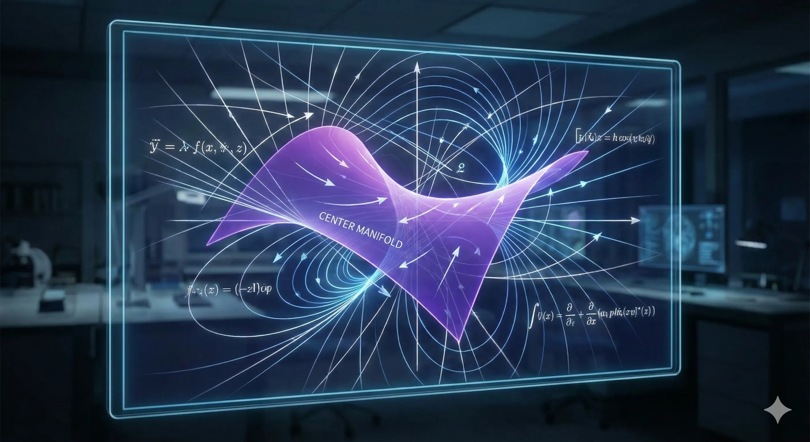
Center Manifold for PDE Dynamics: A Concrete Example

Consider the -dimensional parabolic problem
We study the local dynamics near the trivial solution .
Linear Analysis
Write the equation as
where and . We can find the eigenvalues through the linearization at ,
yielding the eigenvalues: .
Center Subspace () The center subspace corresponds to eigenvalues with zero real part ().
Thus, the center subspace is spanned by the modes and .
Hyperbolic Subspace () The hyperbolic subspace corresponds to eigenvalues with non-zero real parts (). Therefore, the hyperbolic subspace is spanned by all the other modes.
1. Projections
We define the projection operators and onto the center and hyperbolic subspaces, respectively:
The projection operator onto the center subspace for a function , using the standard inner product , is given by
The projection onto the hyperbolic subspace is the complement:
For convenience, we use the projection acting on the Fourier series of a function throughout this article.
Projection onto Center Subspace ()
Projection onto Hyperbolic Subspace ()
2. Substitute the Ansatz
We decompose the solution onto components on the center and hyperbolic subspaces:
where and , and then substitute it into the PDE:
because . Here, and can be expressed using the amplitude and the bases of the center and hyperbolic subspaces:
We project this equation onto and .
Projection onto :
because the -derivative does not change the modes of on the LHS (so ), and , on the RHS. Extracting the coefficient of gives the reduced equation with respect to :
Note: This projection produces another reduced equation that involves by collecting the terms. We are omitting it because it is simply a conjugate copy of the equation. In general, a center subspace spanned by two generic basis functions would result in a -dimensional reduced system.
Projection onto :
Since (because ), this simplifies to:
To summarize, we have now computed the reduced equation on up to the first order
Higher Orders
To close the reduced equation at cubic order , we need at quadratic order . Thus, we can neglect the and terms in the -equation as they are of order and , respectively. Recall that the reduced equation for is:
We expand in the hyperbolic modes:
Now compute each term of the reduced equation.
RHS term :
All terms of are in (modes 0 and ). So .
LHS term : Using the chain rule and the fact that depends on time only through and :
At leading order, . (we only need the linear term from the previous section here because is already second order; higher order corrections to would push the result to ). Thus,
To be very, very precise, we can assume that take the form
in which case the derivatives and becomes explicit. The radius of convergence of this power series is not a concern as the center manifold only makes sense locally.
3: More Substitution and Projections
Assume , , and for some . How do I know that these are all the terms for each ? In other words, what happens if we include another term in one of the ‘s, say, ? In this case, the (constant) terms of the equation becomes
Note that this is the only equation that involves and because the linear operator on the LHS does not change the mode of the input function. The constant term on the RHS only has an term in its coefficient and hence forces . This observation enables us to eliminate most of the terms with zero coefficients.
We solve for by matching terms with the same frequencies. Substitute the ansatz into the reduced equation:
Solve for the Mode k=0:
Substitute :
- LHS term: Using , , and , we have
- LHS term:
- RHS: The constant term in is .
Assemble the equation for :
Solve for the Mode k=2:
Substitute :
- LHS term:
- LHS term:
- RHS: The term in is .
Assemble the equation for :
By symmetry (since is real), .
4. Assemble the Reduced Equation
Return to the equation for :
We analyze the terms inside the bracket that generate the mode.
-
: Contains only modes. No resonance.
-
: Although contains resonating terms, it is of order . Neglect.
-
: This is the interaction term.
The following terms are proportional to :
Substituting the expressions for and found in the previous step:
Substitute these back into the equation:
If we set , the equation becomes
For even higher order expansion of this reduced equation, one can repeat the procedure (substitution, projection, and matching coefficients) based on this order 3 expansion.
As a final reminder, is the coordinate in the center subspace spanned by . So this reduced equation describes the dynamics near the trivial solution . Another note is that should be thought of as the image of under a smooth1 map , i.e., . By inspecting the Taylor expansion of (suppressing for simplicity):
- The first term vanishes because the center manifold passes through the point .
- The second term is zero because the center manifold is tangent to the center subspace at . This is why we can assume is of order in the calculation.
Reference
Local Bifurcations, Center Manifolds, and Normal Forms in Infinite-Dimensional Dynamical Systems by Mariana Haragus and Gérard Iooss.
Footnotes
-
The regularity of the center manifold is whole another topic. Refer to the book above for more details. ↩