Here is a toy problem with a typical saddle-node bifurcation

$$\dot{u} = \mu -u^2$$

that demonstrates the need for continuation method. For each $\mu \in \mathbb{R}_{\geq 0}$ there is an (or two) equilibrium solution $u \equiv \pm\sqrt{\mu}$. Suppose we only know one such fixed point $(u,\mu) = (2,4)$ and wish to find all other equilibria. In practice, discretized differential equations for example, the actual landscape of the dynamical system is often higher dimensional and much more complex than a nice quadratic curve. We employ a basic example here to highlight the core theoretical concepts, avoiding the obfuscation of unnecessary details. The method discussed here applies to a large family of problem of the form $F(v(t))=0$ where $F: \mathbb{R}^{n+1} \to \mathbb{R}^n$ and $v=(u,\mu)$.

Baby Continuation

The naive approach is to increment $\mu$ by small steps towards the left (or right, but the left is the more dangerous direction because it passes through the fold point $(0,0)$). The baby continuation algorithm proceeds as follows:

1. Initialize the continuation by finding a solution $v_0 = (u_0,\mu_0)$ with $F(v_0)=0$.
2. Start loop.
3. Increment in $\mu$: $\mu_1=\mu_0-\delta$.
4. Solve $F(v_1)=0$ for $v_1=(u_1,\mu_1)$ using Newton’s method with $(u_0,\mu_1)$ as the initial guess.
5. Set $v_0 := v_1$.
6. End loop.

As illustrated in the python program below, the baby continuation algorithm fails near the fold point $(u,\mu)=(0,0)$ because it can only continue horizontally to the left and search for solutions vertically (for each newton loop, the $\mu$ value is fixed, so we can only vary $u_0$, in the vertical direction). But there is no solution to be found on the left of the fold point, which causes it to “fall off the cliff”. The newton loop diverges quickly when the supplied initial guess is far away from the true solution, or there is no solution along the specified search route.

The key issue here is that the fixed searching path in the baby continuation makes it impossible to overcome turning points. To resolve this, we implement a path-following strategy capable of negotiating sharp turns, ensuring the solver consistently tracks the bifurcation curve. In other words, this new continuation algorithm adjusts its path adaptively so that it can grab on to the bifurcation curve even near the edge of the cliff.

Pseudo-arclength Continuation

The trick is to view $v=(u,\mu)$ as a single item and, instead of continuing in $\mu$ only, it continues in both spatial and parameter space. The arclength continuation algorithm goes as follows:

1. Initialize the continuation by finding a solution $v_0 = (u_0,\mu_0)$ such that $F(v_0)=0$.
2. Start loop
3. Find the kernel $e$ of $D_u F(v_0)$.
4. Normalize $e$ so that $|e|=1$.
5. Increment $v_0 = v_0 + \delta \cdot e$.
6. Solve $$\begin{align*} F(v_1) &= 0\\ \langle v_1-v_0, e \rangle &= 0 \end{align*}$$ for $v_1=(u_1,\mu_1)$ using Newton’s method with $v_0$ as the initial guess.
7. Set $v_0 := v_1$.
8. End loop.

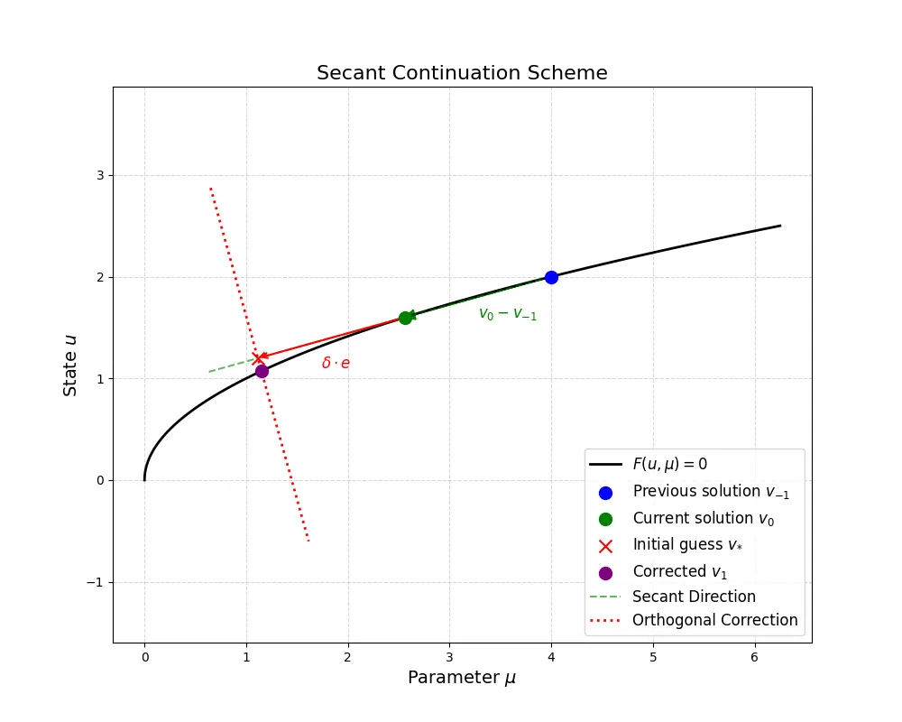
Secant Continuation

Sometimes the kernel $e$ of $D_u F(v_0)$ can be cumbersome to compute. An alternative to a vector $e$ in the arclenth direction is the secant vector, given by $e := v_0 - v_{-1}$ where $v_{-1}$ is the solution found in the previous continuation step. The upside is that we don’t have to go through the hassle computing a kernel; the downside is that now we need to initialize the algorithm with two known solutions (they better be near each other to produce a good secant vector that closely traces the bifurcation curve). We should also keep track of two solutions $v_{-1}$ and $v_0$, instead of just one in the arclength continuation, throughout the continuation.

The secant continuation goes like this:

1. Initialize the continuation by finding a solution $v_{-1} = (u_{-1},\mu_{-1})$ and $v_0 = (u_0,\mu_0)$ such that $F(v_{-1}) = F(v_0) =0$.
2. Start loop
3. Find the secant $e := v_0 - v_{-1}$.
4. Normalize $e$ so that $|e|=1$.
5. Increment $v_* = v_0 + \delta \cdot e$.
6. Solve $$\begin{align*} F(v_1) &= 0\\ \langle v_1-v_*, e \rangle &= 0 \end{align*}$$ for $v_1=(u_1,\mu_1)$ using Newton’s method with $v_0$ as the initial guess.
7. Set $v_{-1} := v_0$ and then $v_0 := v_1$
8. End loop.

The secant continuation is implemented the python notebook below. The results confirm that the algorithm traverses the turning point without divergence, capturing the other solution branch.

The key insight from the arclength/secant continuation is to continue in the direction $e$ that is tangential to the bifurcation curve. Besides solving $F(v)=0$, we added an extra condition $\langle v-v_*, e \rangle = 0$ so that the combined system is still a square system ($\mathbb{R}^{n+1} \to \mathbb{R}^{n+1}$). The vector $v-v_*$ controls the searching route and, together with this condition, ensures that the Newton’s loop always look for solution along a straight line that is orthogonal to the secant line. As a result, there is a much bigger chance of finding an intersection between the searching path and the bifurcation curve near the initial guess $v_*$ provided that the increment rate $\delta$ is sufficiently small.